Gumbel distribution

The Gumbel distribution is a probability distribution of extreme values.

In probability theory and statistics, the Gumbel distribution is used to model the distribution of the maximum (or the minimum) of a number of samples of various distributions.^[1]

Such a distribution might be used to represent the distribution of the maximum level of a river in a particular year if there was a list of maximum values for the past ten years. It is also useful in predicting the chance that an extreme earthquake, flood or other natural disaster will occur.

The Gumbel distribution is a continuous probability distribution. Gumbel distributions are a family of distributions of the same general form. These distributions differ in their location and scale parameters: the mean ("average") of the distribution defines its location, and the standard deviation ("variability") defines the scale.

One recognizes the Gumbel probability density function (PDF) and the Gumbel cumulative distribution function (CDF).

In the PDF, the probability P of a value V to occur between limits A and B, briefly written as P(A<V<B), is found by the area under the PDF curve between A and B.

Example of probability in the PDF

In the figure of the normal probability density function, the values on the horizontal axis should read: μ-3σ, μ-2σ, μ-1σ, μ+1σ, μ+2σ, and μ+3σ respectively. μ = mean, σ = standard deviation. The areas under the curve in the intervals, each with a width of one standard deviation, give the probability of occurrence in those intervals. Example: the probability of a value V to occur in the interval between A=μ+1σ and B=μ+2σ is P(μ+1σ<V<μ+2σ)=13.6% or 0.136

Contrary to the normal distribution, the Gumbel PDF is a-symmetrical and skew to the right.

In the CDF, the probability that a value V is less than A is found directly as the CDF value at A:

${\displaystyle P(V\leq A)=CDF(A)}$.

Example of probability in the CDF

In the Gumbel CDF figure, the red curve indicates that the probability of V to be less than 5 is 0.9 (or 90%), whereas for the dark blue line this probability is 0.7 or 70%

The mathematical expression of the CDF is:

${\displaystyle CDF(A)=e^{-e^{-(A-\mu )/\beta }},}$

where μ is the mode (the value where the probability density function reaches its peak), e is a mathematical constant, about 2.718, and β is a value related to the standard deviation (σ) :

${\displaystyle \beta =\sigma {\sqrt {6}}/\pi ,}$

where π is the Greek symbol for Pi whose value is close to 22/7 or 3.142, and the symbol ${\displaystyle {\sqrt {\,\,}}}$ stands for the square root.

The mode μ can be found from the median M, being the value of A where CDF(A)=0.5, and β:

${\displaystyle \mu =M+\beta \ln \left(\ln 2\right),}$

where ln is the natural logarithm.

The mean, E(x), given by:

${\displaystyle \operatorname {E} (x)=\mu +c\beta ,}$

where ${\displaystyle c}$ = Euler constant ${\displaystyle \approx }$ 0.5772.

In a data series, the parameters mode (μ) and β can be estimated from the average, median and standard deviation. The calculation of the last three quantities is explained in the respective Wiki pages. Then, with the help of formulas given in the previous section, the factors μ and β can be calculated. In this way, the CDF of the Gumbel distribution belonging to the data can be determined and the probability of interesting data values can be found.

In hydrology, the Gumbel distribution is used to analyze such variables as monthly and annual maximum values of daily rainfall and river discharge volumes,^[3] and also to describe droughts.^[4]

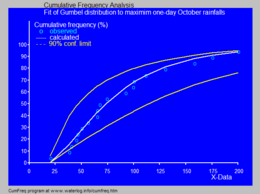
The blue picture illustrates an example of fitting the Gumbel distribution to ranked maximum one-day October rainfalls showing also the 90% confidence belt based on the binomial distribution.

References

[change | change source]- ↑ Gumbel, E.J. 1954. "Statistical theory of extreme values and some practical applications". Applied Mathematics Series, 33. U.S. Department of Commerce, National Bureau of Standards.
- ↑ CumFreq software for distribution fitting
- ↑ Ritzema, H.P., ed. (1994). Frequency and Regression Analysis (PDF). Chapter 6 in: Drainage Principles and Applications, Publication 16, International Institute for Land Reclamation and Improvement (ILRI), Wageningen, The Netherlands. pp. 175–224. ISBN 90-70754-33-9.
- ↑ Burke, E.J.; Perry R.H.J.; Brown, S.J. (2010) "An extreme value analysis of UK drought and projections of change in the future", Journal of Hydrology